Understanding the Adam Optimization Algorithm in Machine Learning
Machine learning and artificial intelligence are some of the most advanced technologies applicable across many industries, including healthcare, finance, transportation, and entertainment. These technologies require powerful algorithms to achieve high accuracy. One such algorithm is the Adam optimization algorithm, which has gained popularity due to its effectiveness and versatility.
This article will delve into the workings of the Adam optimization algorithm, explaining its history, advantages, and applications. We will also compare it with other optimization algorithms and assess its performance on standard datasets like MNIST.
The Basics of Optimization
To understand the Adam algorithm, we need to understand the concept of optimization in machine learning. Optimization involves adjusting the parameters of a machine learning model to minimize or maximize its performance, measured by a loss function. The loss function quantifies the difference between the model's predicted outputs and the actual outputs.
The Adam algorithm, proposed by Diederik Kingma and Jimmy Ba in 2015, is an adaptive optimization method that efficiently updates the model parameters by maintaining a separate learning rate for each parameter.
Advantages of Adam
- Adaptive learning rates: Adam adapts the learning rate for each parameter based on its history of updates, allowing for more efficient convergence.
- Momentum: Incorporates momentum to accelerate the learning process and overcome local minima.
- Combination of algorithms: Merges benefits from AdaGrad and RMSProp to optimize non-stationary data.
Implementation of Adam
The Adam algorithm updates the model parameters by iteratively computing the exponential moving average of the gradients and the squared gradients.
Problem: Optimizing a Simple Quadratic Function
Consider the quadratic function: f(x, y) = x^2 + y^2. This function can be visualized as a 2D
contour plot.
Solution: Using Adam Optimizer
The Adam optimizer efficiently finds the minimum of this function through a structured approach:
- Initialize parameters and moments.
- Iterate through gradient calculations and moment updates.
- Adjust the parameters until convergence.
Code Example
import numpy as np
import matplotlib.pyplot as plt

def loss_function(x, y):
    return x**2 + y**2

def gradient(x, y):
    return np.array([2*x, 2*y])

def adam_optimizer(x, y, alpha=0.1, beta1=0.9, beta2=0.999, epsilon=1e-8):
    m = np.zeros_like(x)
    v = np.zeros_like(x)
    t = 0
    while True:
        t += 1
        grad = gradient(x, y)
        m = beta1 * m + (1 - beta1) * grad
        v = beta2 * v + (1 - beta2) * grad**2
        m_hat = m / (1 - beta1**t)
        v_hat = v / (1 - beta2**t)
        x = x - alpha * m_hat / (np.sqrt(v_hat) + epsilon)
        y = y - alpha * m_hat / (np.sqrt(v_hat) + epsilon)
        loss = loss_function(x, y)
        yield x, y, loss
This code executes the Adam optimizer and visualizes results. Experiment with different learning rates to see how they impact optimization.
Adam Optimizer Visualization
Adjust parameters and see how Adam optimizer converges!
Optimization Algorithm Comparison
Select an optimization algorithm and visualize how it minimizes the loss function:
Train MNIST Model using Adam Optimizer and PyTorch
The MNIST dataset consists of 60,000 training images and 10,000 testing images of handwritten digits (0-9).
- Each image is 28x28 pixels in grayscale.
- Commonly used for benchmarking classification algorithms.
- Developed by Yann LeCun, Corinna Cortes, and Christopher Burges.
It serves as a foundational dataset in deep learning research, often used for training and evaluating neural networks.
Sample MNIST Images
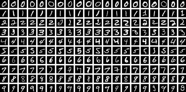
By Suvanjanprasai - Own work, CC BY-SA 4.0, https://commons.wikimedia.org/w/index.php?curid=156115980
            import torch
            from torch import nn
            from tqdm import tqdm

            class NeuralNetwork(nn.Module):
                def __init__(self, input_size, num_classes):
                    """
                    Args:
                        input_size: (1,28,28)
                        num_classes: 10
                    """
                    super(NeuralNetwork, self).__init__()

                    self.layer1 = nn.Sequential(
                        nn.Conv2d(input_size[0], 32, kernel_size=5),
                        nn.ReLU(),
                        nn.MaxPool2d(kernel_size=2))

                    self.layer2 = nn.Sequential(
                        nn.Conv2d(32, 64, kernel_size=5),
                        nn.ReLU(),
                        nn.MaxPool2d(kernel_size=2))

                    self.fc1 = nn.Linear(4 * 4 * 64, num_classes)


                def forward(self, x):
                    """
                    Args:
                        x: (Nx1x28x28) tensor
                    """
                    x = self.layer1(x)
                    x = self.layer2(x)
                    x = x.reshape(x.size(0), -1)
                    x = self.fc1(x)
                    return x

                model = NeuralNetwork((1, 28, 28), 10)

            opts = {
                'lr': 5e-4,
                'epochs': 50,
                'batch_size': 64
            }

            optimizer = torch.optim.Adam(model.parameters(), opts['lr'])
            criterion = torch.nn.CrossEntropyLoss()  # loss function
            train_loader = torch.utils.data.DataLoader(dataset=train_dataset, batch_size=opts['batch_size'], shuffle=True)
            test_loader = torch.utils.data.DataLoader(dataset=test_dataset, batch_size=opts['batch_size'], shuffle=True)

            for epoch in range(opts['epochs']):
                train_loss = []
                for i, (data, labels) in tqdm(enumerate(train_loader), total=len(train_loader)):
                    outputs = model(data)
                    loss = criterion(outputs, labels)
                    optimizer.zero_grad()
                    loss.backward()
                    optimizer.step()
                    train_loss.append(loss.item())
                test_loss = []
                test_accuracy = []
                for i, (data, labels) in enumerate(test_loader):
                    outputs = model(data)
                    _, predicted = torch.max(outputs.data, 1)
                    loss = criterion(outputs, labels)
                    test_loss.append(loss.item())
                    test_accuracy.append((predicted == labels).sum().item() / predicted.size(0))
                print('epoch: {}, train loss: {}, test loss: {}, test accuracy: {}'.format(epoch, np.mean(train_loss), np.mean(test_loss), np.mean(test_accuracy)))
The above code reaches >99% accuracy on the MNIST dataset.